Machine Learning with Tensorflow

Posted on April 10, 2017December 2, 2017 by Bo

Coursera offers an excellent machine learning course by Andrew Ng. The course provides comprehensive coverage of topics ranging from linear regression, through neural networks, support vector machines, to unsupervised learning. It also comes with a number of exercises that are a perfect complement to the lectures. Only completing those exercises gives you a much greater mastery of various techniques. In 2015, Google opened Tensorflow machine learning API. This blog rewrites solutions to problems presented in ML lectures, but not the assignments(!), using Tensorflow. Tensorflow makes solutions to the original ML examples much simpler. However, more importantly, if one has understood Andrew Ng’s course, seeing the same problems expressed using Tensorflow provides a better platform for learning and understanding Tensorflow APIs themselves.

Note: Originally, this blog was to be devoted solely to Andrew Ng’s machine learning course. However, recently I decided to add examples of convolutional neural networks, auto-encoders, recurrent neural networks, etc. If you are just interested in material corresponding to Courser’a course, skip ahead to Linear Regression with Multiple Variables in Tensorflow.

convolutional neural networks, machine learning

Understanding Convolutional Neural Networks

Posted on October 22, 2017October 22, 2017 by Bo

Convolutional neural networks, or CNNs, found applications in computer vision and audio processing. More generally they are suitable for tasks that use a number of features to identify interesting objects, events, sound, etc. The power of CNNs comes from the fact that they can be trained to come up with features that are hard to define by hand. What are “features”, you may ask? It is probably easier to understand this concept through example. Suppose your task is to write a program that can analyze an image of an LCD display and can recognize if the display shows 0 or 1. Thus your program is presented with images that look as follows:

Fig 1. Images representing 0 and 1 on an LCD display

A possible solution would be to convert images to a numeric representation. If 0 was used to represent black pixels, and 1 to represent white pixels, the above images would have numeric representation as shown below:

[[ 1  1  1  1  1]     [[ 0  0  0  0  1]
 [ 1  0  0  0  1]      [ 0  0  0  0  1]
 [ 1  0  0  0  1]      [ 0  0  0  0  1]
 [ 1  0  0  0  1]      [ 0  0  0  0  1]
 [ 1  1  1  1  1]]     [ 0  0  0  0  1]]

Fig 2. Numeric representation of images of 0 and 1

One could make a vertical line a feature (x[i][j] == 1, i = 0 .. 5). Then all the program would have to do is to count the number of features found in each image. If it found two, it would declare that it sees a 0, if it found one, it would output 1. Of course as features go, this one is somewhat weak, as adding 8 to the set of displayed numbers would make the program incorrectly identify it as 0. The point is not, however, to come up with a set of fool-proof features, but rather to illustrate what a feature is.

Back to CNNs. One of the mostly lauded achievements of CNNs is their ability to recognize handwritten digits. It is quite hard to tell what makes a handwritten three a 3. But if you let a CNN look at a sufficient number of handwritten 3s, at some point it comes up, by the virtue of back propagation, with a set of features that, when present, uniquely identify a 3. There is a reasonably comprehensive tutorial on tensorflow.org site that shows how to program a neural network to solve this specific task. My goal is not to repeat it. Instead I go over the concepts that make CNNs such a powerful tool.

In this series of posts I show how to develop a CNN that can recognize all 10 digits shown by a hypothetical LCD display. I start with a simple linear regression to show that automatic derivation of features is not specific to CNNs. By adding a degree of freedom, where digits can appear in a larger image, I show that simple linear regression is not sufficient. One possible approach is to use deep neural networks (DNNs), but they too have limits. The final solution is probably the simplest CNN one can build. Despite its simplicity, it is 100% successful in recognizing all ten digits, regardless of their position on the screen.

convolutional neural networks, linear regression, machine learning

How to recognize a digit

Posted on October 20, 2017October 25, 2017 by Bo

The first task is to train a model so that it can recognize 5 x 5 LCD digits, shown in Fig 1.

zero-to-nine

Fig 1. Images of ten LCD digits

To do this we use a linear regression, which is sufficiently powerful for a task of this complexity.

Each digit is represented as a 5 x 5 array of 0s and 1s. We flatten each one of the arrays into a vector of 25 floats. We stack all vectors forming a 2D array $X_{\mbox{flat}}$ . Next, we compute $X_{\mbox{flat}} W + b$ , where $W$ is a 25 by 10 matrix and $b$ is a vector of size 10.

$\left[ \begin{array}{ccccccc} 1 & 1 & 1 & \cdots & 1 & 1 & 1 \\ 0 & 0 & 0 & \cdots & 0 & 0 & 1 \\ 1 & 1 & 1 & \cdots & 1 & 1 & 1 \\ & & & \ddots & & & \\ 1 & 1 & 1 & \cdots & 1 & 1 & 1 \\ 1 & 1 & 1 & \cdots & 0 & 0 & 1 \end{array} \right] \times \left[ \begin{array}{cccc} w_{0,0} & w_{0,1} & \cdots & w_{0,9} \\ w_{1,0} & w_{1,1} & \cdots & w_{1,9} \\ w_{2,0} & w_{2,1} & \cdots & w_{2,9} \\ & & \ddots & \\ w_{23,0} & w_{23,1} & \cdots & w_{23,9} \\ w_{24,0} & w_{24,1} & \cdots & w_{24,9} \end{array} \right] + \left[ \begin{array}{c} b_0 \\ b_1 \\ \vdots \\ b_9 \end{array} \right]$

The above expression gives us, for each row of $X_{\mbox{flat}}$ , a vector of ten numbers, $y$ referred to as logits. $y_i$ is proportional to the likelihood that the row represents digit $i$ . When training a model, we use gradient descent to nudge the model so that if a row represents, say, a 0, then $y_0$ is greater than $y_1$ … $y_9$ .

We cannot treat $y_i$ as probability, as there is no guarantee that each $y_i$ is between 0 and 1 and the sum of all $y_i$ ‘s adds to 1. However, this can be remedied by using softmax function. A value $h_i$ is expressed as

$\displaystyle h_i = {e^{y_i} \over \sum_{j} e^{y_j}}$

Using softmax converts values y to probabilities h. The goal of training a model is to make sure that when we see an image for, say, 0, the resulting vector $h$ is as close as possible to $[1, 0, 0, 0, 0, 0, 0, 0, 0, 0]$ . This requirement is captured with the help of cross entropy function:

$\displaystyle -\frac{1}{10} \sum_{i = 0}^{10} t_i \lg h_i + (1 - t_i) \lg(1 - h_i)$

Where $t_i$ is the true (desired) value, taking either 1 or 0. Let us express the above using Tensorflow:

img_size = 5
shape_size = 5
kind_count = 10
learning_rate = 0.03
pixel_count = img_size * img_size

x = tf.placeholder(tf.float32,
                   shape=[None, img_size, img_size])
x_flat = tf.reshape(x, [-1, pixel_count])
y_true = tf.placeholder(tf.float32,
                        shape=[None, kind_count])
W = tf.Variable(tf.zeros([pixel_count, kind_count]))
b = tf.Variable(tf.zeros([kind_count]))
y_pred = tf.matmul(x_flat, W) + b
loss_op = tf.reduce_mean(
    tf.nn.softmax_cross_entropy_with_logits(
        labels=y_true, logits=y_pred))
optimizer = tf.train.GradientDescentOptimizer(
    learning_rate)
train_op = optimizer.minimize(loss_op)
correct_prediction = tf.equal(tf.argmax(y_pred, 1),
                              tf.argmax(y_true, 1))
accuracy_op = tf.reduce_mean(
    tf.cast(correct_prediction, tf.float32))

First we set up a few parameters. Initially image size and shape size are going to be the same. This means that the shape completely fills the image. We set the number of kinds of images to 10, so that all ten digits are present. The learning rate defines how fast we follow the slope of the loss function. In our case we chose a conservative 0.03. Choosing a larger value can lead to a faster convergence, but it can also cause us to overshoot the minimum, once we are near it. Lines 7, 8 and 9 create placeholders for input data. Both x and y_true are going to be repeatedly fed batches of images and correct labels for those images. In line 12 we set up the weight matrix. In order to compute $X_{\mbox{flat}} W$ , W must have pixel_count = 25 rows. It has 10 columns (or kind_count) to produce a vector of size 10. The i-th element of that vector is proportional to the likelihood that the given image represents digit i. Line 15 sets up the loss function. It is set as the mean value of softmax expression computed by taking predictions and true labels. Line 18 uses a gradient descent optimizer and line 20 uses it to create a training operation that minimizes the loss function by descending along the gradient of the mean value of the softmax expression. Line 21 computes, for each batch, how many predictions for that batch were correct. Finally, in line 23 we express accuracy as the sum of the correct predictions divided by the total number of predictions. Next comes the training of the model:

sess = tf.InteractiveSession()
sess.run(tf.global_variables_initializer())
batch_maker = BatchMaker(img_data, true_kind, batch_size)
step_nbr = 0
while step_nbr < 5:
  img_batch, label_batch = batch_maker.next()
  train_op.run(feed_dict={x: img_batch, y_true: label_batch})
  step_nbr += 1

We first train the model for five steps. After five steps we print a selection of images. As LCD digits are very regular and fit exactly inside each image, just 5 steps is sufficient to get 60% accuracy:

5-steps

Fig 2. Predictions made by the model after five steps.

The model cannot distinguish between 1, 4, 7 and 9 and between 2 and 3. We continue training until accuracy is 1.

The final matrix W is shown in Fig 3. To better visualize W, we reshape each column of W into a 5 x 5 matrix. Then we normalize each value between -1 and 1. Finally, we plot 1 as red, -1 as blue, 0 as white, and intermediate values as shades of blue or red.

5by5-explain

Fig 3. Matrix W at 100% accuracy.

The red color indicates positive interaction between the matrix and the image, while blue colors indicate negative interaction. Looking at 0, we can see that the model learned to distinguish between 0 and 8 by using negative weights for the line in the middle. For 1, the matrix strongly selects for a vertical line on the left, penalizing at the same time parts that would make the image look like 4, 7 or 9. 3 has positive interaction with almost all but 2 pixels, which would turn 3 into 8. The model did not learn the cleanest features, but it learned enough to tell each digit apart.

Clearly, linear regression can learn a number of features, given a well behaved problem. In the following posts we are going to show how a small change in the problem’s complexity causes linear regression to struggle. The change is to increase the image size, while keeping the digits sizes at 5. Deep neural networks are able to cope with this situation, at the expense of much longer training and much larger models. The final solution, that uses a convolutional neural network, can achieve fast training, 100% accuracy and small model size.

Resources

A Jupyter Notebook with the above code can be found at GitHub’s LCD repository.

machine learning, neural network

Dealing with inexact data

Posted on October 18, 2017October 25, 2017 by Bo

In the previous post we were dealing with an idealized setup. Each 5 by 5 digit fills completely a 5 by 5 image. In real world this is a very unusual occurrence. When processing images there is no guarantee that subjects completely fill them. The subject may be rotated, parts of it might be cut off, shadows may obscure it. The same applies to processing sounds. Ambient noises may be present, the sound we are interested in may not start right at the beginning of the recording, and so on. In this post we are going to show how adding a small degree of uncertainty can defeat an approach based on linear regression. We show how deep neural network can deal with this more complex task, at the expense of a much larger model and longer training time.

Adding uncertainty

In order to simulate a real world setup we are going to slightly alter image generation. Previous image size and shape size were both set to 5. This way each shaped filled perfectly the entire image. There was no uncertainty as to where the image is located. Here we increase the image size to be twice the size of the shape. This leads to shape “jitter”, where the shape can be located anywhere in 10 by 10 grid, as shown in Fig 1.

10by10

Fig 1. LCD digits randomly located on a 10 x 10 grid.

Simple approach

We start by simply modifying img_size variable and running the same linear regression. Somewhat surprisingly, after 5 steps we hit 73% accuracy. When we complete the remaining steps, we reach 100% accuracy. It seems that this approach worked. However, this is not the case. Our linear regression learned perfectly the 100 examples we had. The mistake of the simple approach is not using any test data. Typically, when training a model, it is recommended that about 80% of data is used as training data, and 20% are used as test data. Fortunately, we can easily rectify this. We generate another 50 examples, and evaluate accuracy for those. The result is 8%, or slightly worse than by a random chance. To see why this is the case, let us look at matrix W. Again, we reshape it as a 10 by 10 square, and normalize it within -1 to 1 value. The result is shown in Fig 2.

10by10-explain

Fig 2. Matrix W at the end of training with 100 10×10 images

Now it is obvious that rather than learning how to recognize a given number, linear regression learned the location of each digit. If there is, say, 4 leaning against the left side of the image, it is recognized. However, once it is moved to the location not previously seen, the model lacks the means to recognize it. This is even more obvious if we run the training step with more examples. Rather than maintaining the accuracy, the quality of the solution quickly deteriorates. For example, if we supply 500 rather than 100 examples, the accuracy drops to 54%. Increasing the number of examples to 5,000 drops the accuracy to a dismal 32%. The confusion matrix shows that the only digit that the model learned to recognize is 1.

10by10-confusion

Fig 3. Confusion matrix for 5,000 examples.

Conclusions

Linear model is sufficient only for the most basic case. Even for a highly regular items, such as LCD digits, the model is not capable of learning to recognize them as soon as we permit a small “jitter” in the location of each digit. The above example also shows how important it is to have training and test data sets. Linear regression gave an impression of correctly learning each digits. Only by testing the model against independent test data we discovered that it learned positions of all 100 digits, not how to recognize them. This is reminiscent of case of a neural network that was trained to recognize between tanks camouflaged among trees and just trees (see Section 7.2. An Example of Technical Failure). It seemed to performed perfectly, until it was realized that photos of camouflaged tanks were taken on cloudy days, while all empty forest photos were taken on sunny days. The network learned how to recognize sunny from cloudy days, and knew nothing about tanks.

In the next installment we are going to increase the accuracy by creating a deep neural network.

Resources

You can download the Jupyter notebook from which code snippets and images were presented above from github linreg-large repository.

linear regression, machine learning

Linear Regression with Multiple Variables in Tensorflow

Posted on April 9, 2017May 24, 2017 by Bo

In Lecture 4.1 Linear Regression with multiple variables Andrew Ng shows how to generalize linear regression with a single variable to the case of multiple variables. Andrew Ng introduces a bit of notation to derive a more succinct formulation of the problem. Namely, $n$ features $x_1$ … $x_n$ are extended by adding feature $x_0$ which is always set to 1. This way the hypothesis can be expressed as:

$h_{\theta}(x) = \theta_{0} x_0 + \theta_{1} x_1 + \cdots + \theta_{n} x_n = \theta^T x$

For $m$ examples, the task of linear regression can be expressed as a task of finding vector $\theta$ such that

$\left[ \begin{array}{cccc} \theta_0 & \theta_1 & \cdots & \theta_n \end{array} \right] \times \left[ \begin{array}{ccccc} 1 & 1 & \cdots & 1 \\ x^{(1)}_1 & x^{(2)}_1 & \cdots & x^{(m)}_1 \\ & & \vdots \\ x^{(n)}_m & x^{(n)}_m & \cdots & x^{(n)}_m \\ \end{array} \right]$

is as close as possible to some observed values $y_1, y_2, \cdots, y_m$ . The “as close as possible” typically means that the mean sum of square errors between $h_{\theta}(x^{(i)})$ and $y_i$ for $i \in [1, m]$ is minimized. This quantity is often referred to as cost or loss function:

$J(\theta) = \dfrac{1}{2 m} \sum_{i=1}^{m} \left( h_{\theta}(x^{(i)}) - y_i\right)^2$

To express the above concepts in Tensorflow, and more importantly, have Tensorflow find $\theta$ that minimizes the cost function, we need to make a few adjustments. We rename vector $\theta$ , as w. We are not using $x_0 = 1$ . Instead, we use a tensor of size 0 (also known as scalar), called b to represent $x_0$ . As it is easier to stack rows than columns, we form matrix $X$ , in such a way that the i-th row is the i-th sample. Our formulation thus has the form

$h_{w,b}(X) = \left[ \begin{array}{ccc} \text{---} & (x^{(1)})^T & \text{---} \\ \text{---} & (x^{(2)})^T & \text{---} \\ & \vdots & \\ \text{---} & (x^{(m)})^T & \text{---} \end{array} \right] \times \left[ \begin{array}{c} w_1 \\ w_2 \\ \vdots \\ w_m \end{array} \right] + b$

This leads to the following Python code:

X_in = tf.placeholder(tf.float32, [None, n_features], "X_in")
w = tf.Variable(tf.random_normal([n_features, 1]), name="w")
b = tf.Variable(tf.constant(0.1, shape=[]), name="b")
h = tf.add(tf.matmul(X_in, w), b)

We first introduce a tf.placeholder named X_in. This is how we supply data into our model. Line 2 creates a vector w corresponding to $\theta$ . Line 3 creates a variable b corresponding to $x_0$ . Finally, line 4 expresses function h as a matrix multiplication of X_in and w plus scalar b.

y_in = tf.placeholder(tf.float32, [None, 1], "y_in")
loss_op = tf.reduce_mean(tf.square(tf.subtract(y_in, h)),
                         name="loss")
train_op = tf.train.GradientDescentOptimizer(0.3).minimize(loss_op)

To define the loss function, we introduce another placeholder y_in. It holds the ideal (or target) values for the function h. Next we create a loss_op. This corresponds to the loss function. The difference is that, rather than being a function directly, it defines for Tensorflow operations that need to be run to compute a loss function. Finally, the training operation uses a gradient descent optimizer, that uses learning rate of 0.3, and tries to minimize the loss.

Now we have all pieces in place to create a loop that finds w and b that minimize the loss function.

with tf.Session() as sess:
    sess.run(tf.global_variables_initializer())
    for batch in range(1000):
        sess.run(train_op, feed_dict={
            X_in: X_true,
            y_in: y_true
        })
    w_computed = sess.run(w)
    b_computed = sess.run(b)

In line 1 we create a session that is going to run operations we created before. First we initialize all global variables. In lines 3-7 we repeatedly run the training operation. It computes the value of h based on X_in. Next, it computes the current loss, based on h, and y_in. It uses the data flow graph to compute derivatives of the loss function with respect to every variable in the computational graph. It automatically adjusts them, using the specified learning rate of 0.3. Once the desired number of steps has been completed, we record the final values of vector w and scalar b computed by Tensorflow.

To see how well Tensorflow did, we print the final version of computed variables. We compare them with ideal values (which for the purpose of this exercise were initialized to random values):

print "w computed [%s]" % ', '.join(['%.5f' % x for x in w_computed.flatten()])
print "w actual   [%s]" % ', '.join(['%.5f' % x for x in w_true.flatten()])
print "b computed %.3f" % b_computed
print "b actual  %.3f" % b_true[0]

w computed [5.48375, 90.52216, 48.28834, 38.46674]
w actual   [5.48446, 90.52165, 48.28952, 38.46534]
b computed -9.326
b actual  -9.331

Resources

You can download the Jupyter notebook with the above code from a github linear regression repository.

linear regression, machine learning

Multiple Variable Linear Regression using Tensorflow Layers

Posted on April 8, 2017October 23, 2017 by Bo

In version 1.0 of Tensorflow released in Feb 2017 a higher level APIs, called layers, were added. These allow a reduction in the amount of boilerplate code one has to write. For example, for linear regression with $n$ features we would always create a matrix $X$ and vector $y$ represented by placeholders. We would always create variables representing weights and biases, etc., and so on. By using layers this can be avoided. Instead, we need to focus on describing and supplying data to a regressor. Let us rewrite linear regression using layers. The code is shown below:

x_feature = tf.contrib.layers.real_valued_column('X', 4)
regressor = tf.contrib.learn.LinearRegressor(
  [x_feature],
  optimizer=tf.train.GradientDescentOptimizer(0.3))
regressor.fit(
  input_fn=create_training_fn(m_examples, w_true, b_true),
  steps=500)
eval_dict = regressor.evaluate(
  input_fn=create_training_fn(10, w_true, b_true), steps=1)

First we describe our features. In our simple case we create a real valued feature, named X, 4 columns wide. We could have created four features x₁ … x₄. However, this would make input function more complex. Next, we create a linear regressor. We pass feature columns to it. It must be an iterable. Otherwise it will fail with fairly mysterious errors. The second parameter is the optimizer. We chose to rely on the same gradient descent optimizer as in the last example. Having created the regressor we train it, by calling fit method. This is done with the help of the input function that feeds labeled data into it. We run it for 500 steps. Finally, we evaluate how well the regressor fits the data. In real application, the last step should be called with data not included in the training set.

The input function must return a pair. The first element of the pair must be a map from feature names to feature values. The second element must be the target values (i.e., labels) that the regressor is learning. In our case the function is fairly simple, as shown below:

def create_training_fn(m, w, b):
  def training_fn_():
    X = np.random.rand(m, w.shape[0])
    return ({'X': tf.constant(X)},
            tf.constant(np.matmul(X, w) + b))
  return training_fn_

It generates a random set of input data, X, and computes the target value as $X w + b$ . In real applications this function can be arbitrarily complex. It could, for example, read data and labels from files, returning a fixed number of rows at a time.

Last, let us see how well the LinearRegressor did. Typically, one has just the loss function as the guide. However, for us, we also know w and b. Thus we can compare them with what the regressor computed, by fetching regressor’s variables:

print "loss", eval_dict['loss']
print "w true ", w_true.T[0]
print "w found", regressor.get_variable_value('linear/X/weight').T[0]
print "b true  %.4f" % b_true[0]
print "b found", regressor.get_variable_value('linear/bias_weight')[0]

loss 8.81575e-06
w true  [ 1.7396  62.2283  59.7082  6.9788]
w found [ 1.7304  62.2178  59.6973  6.9751]
b true  -4.7938
b found -4.77659

Both the weights and the bias are very close to the one we used to train the regressor.

It is worth mentioning that regressors also offer a way of tracking internal state that can be used to analyze their behavior using TensorBoard. There are also methods that allow regressor’s state to be saved and later restored. Finally, the predict function can be used to compute regressor output, for any unlabeled input.

machine learning

Computing XNOR with a Neural Network

Posted on April 7, 2017May 24, 2017 by Bo

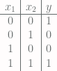
This tutorial shows how to use Tensorflow to create a neural network that mimics $\neg (x_1 \oplus x_2)$ function. This function, abbreviated as XNOR, returns 1 only if $x_1$ is equal to $x_2$ . The values are summarized in the table below:

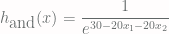
$\begin{array}{c|c|c} x_1 & x_2 & y \\ \hline 0 & 0 & 1 \\ 0 & 1 & 0 \\ 1 & 0 & 0 \\ 1 & 1 & 1 \end{array}$

Andrew Ng shows in Lecture 8.5: Neural Networks – Representation how to construct a single neuron that can emulate a logical AND operation. The neuron is considered to act like a logical AND if it outputs a value close to 0 for (0, 0), (0, 1), and (1, 0) inputs, and a value close to 1 for (1, 1). This can be achieved as follows:

$h_{\mbox{and}}(x)=\dfrac{1}{e^{30 - 20x_1 - 20x_2}}$

To recreate the above in tensorflow we first create a function that takes theta, a vector of coefficients, together with x1 and x2. We use the vector to create three constants, represented by tf.constant. The first one is the bias unit. The next two are used to multiply x1 and x2, respectively. The expression is then fed into a sigmoid function, implemented by tf.nn.sigmoid.

Outside of the function we create two placeholders. For Tensorflow a tf.placeholder is an operation that is fed data. These are going to be our x1 and x2 variables. Next we create a h_and operation by calling the MakeModel function with the coefficient vector as suggested by Andrew Ng.

def MakeModel(theta, x1, x2):
  h = tf.constant(theta[0]) + \
    tf.constant(theta[1]) * x1 + tf.constant(theta[2]) * x2
  return tf.nn.sigmoid(h)

x1 = tf.placeholder(tf.float32, name="x1")
x2 = tf.placeholder(tf.float32, name="x2")
h_and = MakeModel([-30.0, 20.0, 20.0], x1, x2)

We can then print the values to verify that our model works correctly. When creating Tensorflow operations, we do not create an actual program. Instead, we create a description of the program. To execute it, we need to create a session to run it:

with tf.Session() as sess:
  print " x1 | x2 |  g"
  print "----+----+-----"
  for x in range(4):
    x1_in, x2_in = x &amp;amp; 1, x &amp;gt; 1
    print " %2.0f | %2.0f | %3.1f" % (
        x1_in, x2_in, sess.run(h_and, {x1: x1_in, x2: x2_in}))

The above code produces the following output, confirming that we have correctly coded the AND function:

  x1| x2 |  g
----+----+-----
  0 |  0 | 0.0
  0 |  1 | 0.0
  1 |  0 | 0.0
  1 |  1 | 1.0

To get a better understanding of how a neuron, or more precisely, a sigmoid function with a linear input, emulates a logical AND, let us plot its values. Rather than just using four points, we compute its values for a set of 20 x 20 points from the range [0, 1]. First, we define a function that, for a given input function (a tensor) and a linear space, computes values of returned by the function (a tensor) when fed points from the linear space.

def ComputeVals(h, span):
    vals = []
    with tf.Session() as sess:
        for x1_in in span:
            vals.append([
                sess.run(h, feed_dict={
                  x1: x1_in, x2: x2_in}) for x2_in in span
            ])
    return vals

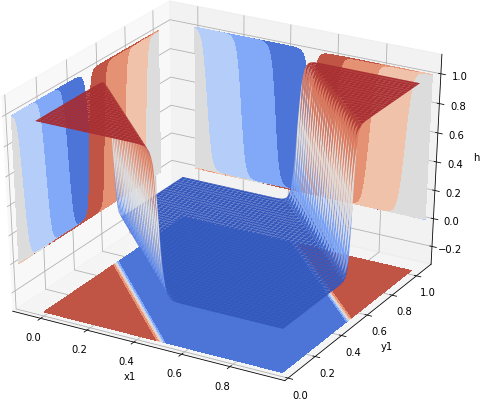
This is a rather inefficient way of doing this. However, at this stage we aim for clarity not efficiency. To plot values computed by the h_and tensor we use matplotlib. The result can be seen in Fig 1. We use coolwarm color map, with blue representing 0 and red representing 1.

h_and

Fig 1. Values of a neuron emulating the AND gate

Having created a logical AND, let us apply the same approach, and create a logical OR. Following Andrew Ng’s lecture, the bias is set to -10.0, while we use 20.0 as weights associated with x1 and x2. This has the effect of generating an input larger than or equal 10.0, if either x1 or x2 are 1, and -10, if both are zero. We reuse the same MakeModel function. We pass the same x1 and x2 as input, but change vector theta to [-10.0, 20.0, 20.0]

h_or = MakeModel([-10.0, 20.0, 20.0], x1, x2)
or_vals = ComputeVals(h_or, span)

When plotted with matplotlib we see the graph shown in Fig 2.

Fig 2. Values of a neuron emulating the OR gate

The negation can be crated by putting a large negative weight in front of the variable. Andrew Ng’s chose 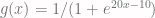$10 - 20x$ . This way $g(x)=1/(1 + e^{20x - 10})$ returns $0.00005$ for $latex x = 1$ and $0.99995$ for $x = 0$ . By using −20 with both x1 and x2 we get a neuron that produces a logical and of negation of both variables, also known as the NOR gate: $h_{nor} = 1/(1+e^{-(10 - 20x1 - 20x2)})$ .

h_nor = MakeModel([10.0, -20.0, -20.0], x1, x2)
nor_vals = ComputeVals(h_nor, span)

The plot of values of our h_nor function can be seen in Fig 3.

nor

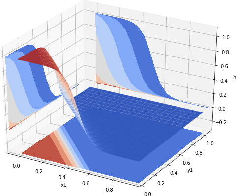
Fig 3. Value of a neuron emulating the NOR gate

With the last gate, we have everything in place. The first neuron generates values close to one when both x1 and x2 are 1, the third neuron generates value close to one when x1 and x2 are close to 0. Finally, the second neuron can perform a logical OR of values generated from two neurons. Thus our xnor neuron can be constructed by passing h_and and h_nor as inputs to h_or neuron. In Tensorflow this simply means that rather than passing x1 and x2 placeholders, when constructing h_or function, we pass h_and and h_nor tensors:

h_xnor = MakeModel([-10.0, 20.0, 20.0], h_nor, h_and)
xnor_vals = ComputeVals(h_xnor, span)

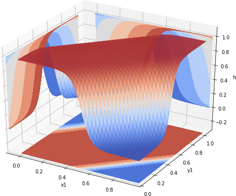
Again, to see what is happening, let us plot the values of h_xnor over the [0, 1] range. These are shown in Fig 4.

xnor
Fig 4. Value of a neural net emulating XNOR gate

In a typical Tensorflow application we would not see only constants being used to create a model. Instead constants are used to initialize variables. The reason we could use only constants is that we do not intend to train the model. Instead we already knew, thanks to Andrew Ng, the final values of all weights and biases.

Finally, the solution that we gave is quite inefficient. We will show next how by vectorising it one can speed it up by a factor of over 200 times. This is not an insignificant number, considering how simple our model is. In larger models vectorization can give us even more dramatic improvements.

Resources

You can download the Jupyter notebook from which code snippets were presented above from github xnor-basic repository.

machine learning

Vectorized XNOR

Posted on April 6, 2017October 23, 2017 by Bo

In the previous post we have showed how to encode XNOR function using a two layers deep neural net. The first layer consists of the NOR and AND gates. The second layer is a single OR gate. The Tensorflow implementation we developed is rather inefficient. This is due to the fact that all computations are done on individual variables. A better way is to create the model so that each layer of the neural net can be computed for a batch of inputs as matrix operations. The input to the first sigmoid function can be computed as follows:

$\left(\begin{array}{cc}x_1^{(1)} & x_2^{(1)} \\ x_1^{(2)} & x_2^{(2)} \\ \cdots \\ x_1^{(m)} & x_2^{(m)} \end{array}\right) \left(\begin{array}{cc} w_{11} & w_{12} \\ w_{21} & w_{22}\end{array}\right) + \left(\begin{array}{cc}b_1 & b_2\end{array}\right)$

This leads to the following model:

X = tf.placeholder(tf.float32, [None, 2], name="X")
W1 = tf.constant([[20.0, -20.0], [20.0, -20.0]])
b1 = tf.constant([-30, 10])
and_nor = tf.sigmoid(tf.add(tf.matmul(X, W1), b1))
W2 = tf.constant([[20.0], [20.0]])
b2 = tf.constant([-10.0])
h_xnor_fast = tf.sigmoid(tf.add(tf.matmul(and_nor, W2),b2))

X representing x1 and x2, has unrestricted first dimension. This allows us to specify arbitrary many inputs. The first layer also computes both AND and NOR gates in a single computation. The second layer takes a single input, the previous layer, and again computes the output in two matrix operation. The function that computes values also undergoes changes

def ComputeValsFast(h, span):
  x1, x2 = np.meshgrid(span, span)
  X_in = np.column_stack([x1.flatten(), x2.flatten()])
  with tf.Session() as sess:
    return np.reshape(sess.run(h, feed_dict={X: X_in}), x1.shape)

It takes the vector that defines a space of input values, flattens it and stacks it as two columns. Then all values can be computed as a single call to sess.run(), followed by the reshaping operation. The difference? The original operation on a MacBook Air run in about 3.07s per loop. The reformulated, so-called fast version, runs in 14.5ms per loop. This level of speed allows us to recompute values of the optimized xor for 10,000, rather than the original 400 points leading to the image shown in Fig 1.

xnor-hd
Fig 1. 100 x 100 XNOR values computed by a neural net.

Resources

You can download the Jupyter notebook from which code snippets were presented above from github xnor-fast repository.

machine learning, neural network

Training neural net to emulate XNOR

Posted on March 31, 2017October 23, 2017 by Bo

In the last two posts we have shown how to encode, using Tensorflow, a neural network that behaves like the XNOR gate. However, it is a very unusual that we know, ahead of time, weights and biases. A much more common scenario is when we have number of inputs and the corresponding values, and wish to train a neural net to produce for each input the appropriate value. For us the inputs are (0, 0), (0, 1), (1, 0) and (1, 1). The values are 1, 0, 0, and 1. We have seen that a 2 layer deep neural network can emulate XNOR with high fidelity. Thus we could just create a 2 layer deep, 3 neuron network and attempt to train it. To facilitate some level of experimentation we create a function that produces a fully connected neural network layer.

def CreateLayer(X, width):
    W = tf.get_variable("W", [X.get_shape()[1].value, width], tf.float32)
    b = tf.get_variable("b", [width], tf.float32)
    return tf.nn.sigmoid(tf.add(tf.matmul(X, W), b))

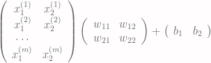
The function creates $X \times W + b$ input to a layer of neurons. Using $X \times W$ instead $W \times X$ allows us to specify $n$ inputs (features) as a $m \times n$ matrix. This is often easier than representing inputs as $m$ columns each $n$ high. Also, rather than creating variables directly, with tf.Variable, we use tf.get_variable. This allows variable sharing, as explained in Sharing Variables. It also can enhance display of the computation graph in TensorBoard, as explained in Hands on TensorBoard presentation.

We also create a training operation and a loss function that allows us to assess how well the current network is doing. Tensorflow offers a whole array of optimizers, but tf.train.AdamOptimizer is often a good choice. In order for the optimizer to push variables to a local minima we must create an optimizer operation. This is done by calling minimize method with a loss function. The loss function tells the optimizer how far it is from the ideal solution. We use the mean of squared errors as our loss function.

def CreateTrainigOp(model, learning_rate, labels):
    loss_op = tf.reduce_mean(tf.square(tf.subtract(model, labels)))
    train_op = tf.train.AdamOptimizer(learning_rate).minimize(loss_op)
    return train_op, loss_op

The above function returns the training and loss operations. The latter is used to track progress of the model towards the optimum. The final piece of code that needs to be written is the training code.

g = tf.Graph()
with g.as_default():
  X = tf.placeholder(tf.float32, [None, 2], name="X")
  y = tf.placeholder(tf.float32, [None, 1], name="y")
  with tf.variable_scope("layer1"):
    z0 = CreateLayer(X, 2)
  with tf.variable_scope("layer2"):
    z1 = CreateLayer(z0, 1)
  with tf.variable_scope("xnor"):
    training_op, loss_op = CreateTrainigOp(z1, 0.03, y)
  init_op = tf.global_variables_initializer()
  saver = tf.train.Saver()

X and y (line 3-4) are placeholders, which are going to be seeded with inputs and desired outputs. We specify the first dimension to be None to allow for arbitrary number of rows. In lines 5 – 10 we create a model. It consists of two, fully connected layers. The first layer has 2 neurons, the second consists of a single neuron. X is the input to the first layer, while the output of the first layer, z0, is the input to the second layer. The output of the second layer, z1 is what we wish to train to behave like the XNOR gate. To do so, in lines 9 and 10 we create a training operation and a loss op. Finally we create an operation to initialize all global variables and a session saver.

writer = tf.summary.FileWriter("/tmp/xnor_log", g)
loss_summ = tf.summary.scalar("loss", loss_op)

Before we run the training step we create a summary writer. We are going to use it to track the loss function. It can also be used to track weights, biases, images, and audio inputs. It also is an invaluable tool for visualizing data flow graph. The graph for our specific example is shown in Fig 1.

Fig 1. Data flow graph as rendered by tensorboard

In order to train our model we create two arrays representing features and labels (input values and the desired output). The training itself is done for 5,000 steps by the for loop. We feed the session all inputs and desired values, and run a training operation. What this does it runs the feed forward steps to compute z1 for the given inputs, weights and biases. These are then compared, using the loss function to the ideal responses, represented by y from these Tensorflow computes contributions all weights and biases make to the loss function. It uses the learning rate 0.03 to adjust them to make the loss smaller.

X_train = np.array([[0, 0], [0, 1], [1, 0], [1, 1],])
y_train = np.array([[1], [0], [0], [1]])

sess = tf.Session(graph=g)
sess.run(init_op)
for step in xrange(5000):
    feed_dict = {X: X_train, y: y_train}
    sess.run(training_op, feed_dict=feed_dict)
    if step % 10 == 0:
        writer.add_summary(
            sess.run(loss_summ, feed_dict=feed_dict), step)
save_path = saver.save(sess, '/tmp/xnor.ckpt')
sess.close()
print "Model trained. Session saved in", save_path

Once the training is complete we save the state of the session, close it and print the location of the single session checkpoint. The loss function, as recorded by the summary file writer, and rendered by TensorBoard, is shown in Fig 2.

loss
Fig 2. Loss function plotted by tensorboard.

At the end of the training it the loss function has the value of 0.000051287. It was still dropping but very slowly. In the next post we show how to restore the session and plot the loss function as well as the output of the trained neural network.

Resources

The Jupyter notebook that implements the above discussed functionality is xnor-train.ipynb in the xnor-train project.

machine learning, neural network

Using XNOR trained model

Posted on March 24, 2017October 23, 2017 by Bo

In the previous post we have described how to train a simple neural net to emulate the XNOR gate. The results of the training are saved as a solitary session checkpoint. In this post we show how to re-create the model, load the weights and biases saved to the checkpoint and finally plot the surface generated by the neural net over [0,1] x [0,1] surface.

tf.reset_default_graph()
X = tf.placeholder(tf.float32, [None, 2], name="X")
with tf.variable_scope("layer1"):
  z0 = CreateLayer(X, 2)
with tf.variable_scope("layer2"):
  z1 = CreateLayer(z0, 1)

We start by re-creating the model. For convenience, we added tf.reset_default_graph() call. Otherwise an attempt to re-execute this particular Jupyter cell results in error. Just like during the training method we create a placeholder for input values. We do not need, however, a placeholder for the desired values, y. Next, we re-create the neural network, creating two, fully connected layers.

saver = tf.train.Saver()
sess = tf.Session()
saver.restore(sess, "/tmp/xnor.ckpt")

The next three lines create a saver, a session, and restore the state of the session from the saved checkpoint. In particular, this restores the trained values for weights and biases.

span = np.linspace(0, 1, 100)
x1, x2 = np.meshgrid(span, span)
X_in = np.column_stack([x1.flatten(), x2.flatten()])
xnor_vals = np.reshape(
    sess.run(z1, feed_dict={X: X_in}), x1.shape)
sess.close()
PlotValues(span, xnor_vals)

The final piece of the code creates a 100 x 100 mesh of points from the [0,1] x [0,1] range. These are then reshaped to the shape required by X placeholder. Next, the session runs z1 operation, which returns values computed by the neural net for the given input X. As these are returned as 10,000 x 1 vector, we reshape them back to the grid shape before assigning them to xnor_vals. Once the session is closed, the values are plotted, resulting in surface shown in Fig 1.

xnor-trained-hd
Fig 1. Values produced by the trained neural net

The surface significantly different from the plots produced by Andrew Ng’s neural network. However, both of them agree at the extremes. To plot the values at the corner of the plane we run the following code:

print " x1| x2| XNOR"
print "---+---+------"
print " 0 | 0 | %.3f" % xnor_vals[0][0]
print " 0 | 1 | %.3f" % xnor_vals[0][-1]
print " 1 | 0 | %.3f" % xnor_vals[-1][0]
print " 1 | 1 | %.3f" % xnor_vals[-1][-1]

The result is shown below

  x1 | x2| XNOR
 ---+---+------
  0 | 0 | 0.996
  0 | 1 | 0.005
  1 | 0 | 0.004
  1 | 1 | 0.997

As it can be seen, for the given inputs the training produced the desired output. The network produces values close to 1 for (0, 0) and (1, 1) and values close to 0 for (0, 1) and (1, 0). If the above code is run multiple times, since weights and biases are initialized randomly, sometimes the trained network produces results that resemble those produced by Andrew Ng’s network.