convolutional neural networks, machine learning

Understanding Convolutional Neural Networks

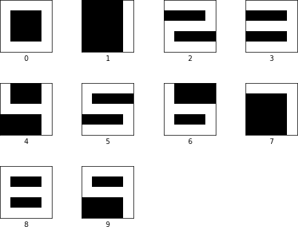
Convolutional neural networks, or CNNs, found applications in computer vision and audio processing. More generally they are suitable for tasks that use a number of features to identify interesting objects, events, sound, etc. The power of CNNs comes from the fact that they can be trained to come up with features that are hard to define by hand. What are “features”, you may ask? It is probably easier to understand this concept through example. Suppose your task is to write a program that can analyze an image of an LCD display and can recognize if the display shows 0 or 1. Thus your program is presented with images that look as follows:

Fig 1. Images representing 0 and 1 on an LCD display

A possible solution would be to convert images to a numeric representation. If 0 was used to represent black pixels, and 1 to represent white pixels, the above images would have numeric representation as shown below:

[[ 1  1  1  1  1]     [[ 0  0  0  0  1]
 [ 1  0  0  0  1]      [ 0  0  0  0  1]
 [ 1  0  0  0  1]      [ 0  0  0  0  1]
 [ 1  0  0  0  1]      [ 0  0  0  0  1]
 [ 1  1  1  1  1]]     [ 0  0  0  0  1]]

Fig 2. Numeric representation of images of 0 and 1

One could make a vertical line a feature (x[i][j] == 1, i = 0 .. 5). Then all the program would have to do is to count the number of features found in each image. If it found two, it would declare that it sees a 0, if it found one, it would output 1. Of course as features go, this one is somewhat weak, as adding 8 to the set of displayed numbers would make the program incorrectly identify it as 0. The point is not, however, to come up with a set of fool-proof features, but rather to illustrate what a feature is.

Back to CNNs. One of the mostly lauded achievements of CNNs is their ability to recognize handwritten digits. It is quite hard to tell what makes a handwritten three a 3. But if you let a CNN look at a sufficient number of handwritten 3s, at some point it comes up, by the virtue of back propagation, with a set of features that, when present, uniquely identify a 3. There is a reasonably comprehensive tutorial on tensorflow.org site that shows how to program a neural network to solve this specific task. My goal is not to repeat it. Instead I go over the concepts that make CNNs such a powerful tool.

In this series of posts I show how to develop a CNN that can recognize all 10 digits shown by a hypothetical LCD display. I start with a simple linear regression to show that automatic derivation of features is not specific to CNNs. By adding a degree of freedom, where digits can appear in a larger image, I show that simple linear regression is not sufficient. One possible approach is to use deep neural networks (DNNs), but they too have limits. The final solution is probably the simplest CNN one can build. Despite its simplicity, it is 100% successful in recognizing all ten digits, regardless of their position on the screen.

convolutional neural networks, linear regression, machine learning

How to recognize a digit

The first task is to train a model so that it can recognize 5 x 5 LCD digits, shown in Fig 1.

zero-to-nine

Fig 1. Images of ten LCD digits

To do this we use a linear regression, which is sufficiently powerful for a task of this complexity.

Each digit is represented as a 5 x 5 array of 0s and 1s. We flatten each one of the arrays into a vector of 25 floats. We stack all vectors forming a 2D array X_{\mbox{flat}}. Next, we compute X_{\mbox{flat}} W + b , where W is a 25 by 10 matrix and b is a vector of size 10.

\left[ \begin{array}{ccccccc} 1 & 1 & 1 & \cdots & 1 & 1 & 1 \\ 0 & 0 & 0 & \cdots & 0 & 0 & 1 \\ 1 & 1 & 1 & \cdots & 1 & 1 & 1 \\ & & & \ddots & & & \\ 1 & 1 & 1 & \cdots & 1 & 1 & 1 \\ 1 & 1 & 1 & \cdots & 0 & 0 & 1 \end{array} \right] \times \left[ \begin{array}{cccc} w_{0,0} & w_{0,1} & \cdots & w_{0,9} \\ w_{1,0} & w_{1,1} & \cdots & w_{1,9} \\ w_{2,0} & w_{2,1} & \cdots & w_{2,9} \\ & & \ddots & \\ w_{23,0} & w_{23,1} & \cdots & w_{23,9} \\ w_{24,0} & w_{24,1} & \cdots & w_{24,9} \end{array} \right] + \left[ \begin{array}{c} b_0 \\ b_1 \\ \vdots \\ b_9 \end{array} \right]

The above expression gives us, for each row of X_{\mbox{flat}}, a vector of ten numbers, y referred to as logits. y_i is proportional to the likelihood that the row represents digit i
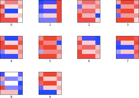
. When training a model, we use gradient descent to nudge the model so that if a row represents, say, a 0, then y_0 is greater than y_1y_9.

We cannot treat y_i as probability, as there is no guarantee that each y_i is between 0 and 1 and the sum of all y_i‘s adds to 1. However, this can be remedied by using softmax function. A value h_i is expressed as

\displaystyle h_i = {e^{y_i} \over \sum_{j} e^{y_j}}

Using softmax converts values y to probabilities h. The goal of training a model is to make sure that when we see an image for, say, 0, the resulting vector h is as close as possible to [1, 0, 0, 0, 0, 0, 0, 0, 0, 0]. This requirement is captured with the help of cross entropy function:

\displaystyle -\frac{1}{10} \sum_{i = 0}^{10} t_i \lg h_i + (1 - t_i) \lg(1 - h_i)

Where t_i is the true (desired) value, taking either 1 or 0. Let us express the above using Tensorflow:

img_size = 5
shape_size = 5
kind_count = 10
learning_rate = 0.03
pixel_count = img_size * img_size

x = tf.placeholder(tf.float32,
                   shape=[None, img_size, img_size])
x_flat = tf.reshape(x, [-1, pixel_count])
y_true = tf.placeholder(tf.float32,
                        shape=[None, kind_count])
W = tf.Variable(tf.zeros([pixel_count, kind_count]))
b = tf.Variable(tf.zeros([kind_count]))
y_pred = tf.matmul(x_flat, W) + b
loss_op = tf.reduce_mean(
    tf.nn.softmax_cross_entropy_with_logits(
        labels=y_true, logits=y_pred))
optimizer = tf.train.GradientDescentOptimizer(
    learning_rate)
train_op = optimizer.minimize(loss_op)
correct_prediction = tf.equal(tf.argmax(y_pred, 1),
                              tf.argmax(y_true, 1))
accuracy_op = tf.reduce_mean(
    tf.cast(correct_prediction, tf.float32))

First we set up a few parameters. Initially image size and shape size are going to be the same. This means that the shape completely fills the image. We set the number of kinds of images to 10, so that all ten digits are present. The learning rate defines how fast we follow the slope of the loss function. In our case we chose a conservative 0.03. Choosing a larger value can lead to a faster convergence, but it can also cause us to overshoot the minimum, once we are near it. Lines 7, 8 and 9 create placeholders for input data. Both x and y_true are going to be repeatedly fed batches of images and correct labels for those images. In line 12 we set up the weight matrix. In order to compute X_{\mbox{flat}} W, W must have pixel_count = 25 rows. It has 10 columns (or kind_count) to produce a vector of size 10. The i-th element of that vector is proportional to the likelihood that the given image represents digit i. Line 15 sets up the loss function. It is set as the mean value of softmax expression computed by taking predictions and true labels. Line 18 uses a gradient descent optimizer and line 20 uses it to create a training operation that minimizes the loss function by descending along the gradient of the mean value of the softmax expression. Line 21 computes, for each batch, how many predictions for that batch were correct. Finally, in line 23 we express accuracy as the sum of the correct predictions divided by the total number of predictions. Next comes the training of the model:

sess = tf.InteractiveSession()
sess.run(tf.global_variables_initializer())
batch_maker = BatchMaker(img_data, true_kind, batch_size)
step_nbr = 0
while step_nbr < 5:
  img_batch, label_batch = batch_maker.next()
  train_op.run(feed_dict={x: img_batch, y_true: label_batch})
  step_nbr += 1

We first train the model for five steps. After five steps we print a selection of images. As LCD digits are very regular and fit exactly inside each image, just 5 steps is sufficient to get 60% accuracy:

5-steps

Fig 2. Predictions made by the model after five steps.

The model cannot distinguish between 1, 4, 7 and 9 and between 2 and 3. We continue training until accuracy is 1.

The final matrix W is shown in Fig 3. To better visualize W, we reshape each column of W into a 5 x 5 matrix. Then we normalize each value between -1 and 1. Finally, we plot 1 as red, -1 as blue, 0 as white, and intermediate values as shades of blue or red.

5by5-explain

Fig 3. Matrix W at 100% accuracy.

The red color indicates positive interaction between the matrix and the image, while blue colors indicate negative interaction. Looking at 0, we can see that the model learned to distinguish between 0 and 8 by using negative weights for the line in the middle. For 1, the matrix strongly selects for a vertical line on the left, penalizing at the same time parts that would make the image look like 4, 7 or 9. 3 has positive interaction with almost all but 2 pixels, which would turn 3 into 8. The model did not learn the cleanest features, but it learned enough to tell each digit apart.

Clearly, linear regression can learn a number of features, given a well behaved problem. In the following posts we are going to show how a small change in the problem’s complexity causes linear regression to struggle. The change is to increase the image size, while keeping the digits sizes at 5. Deep neural networks are able to cope with this situation, at the expense of much longer training and much larger models. The final solution, that uses a convolutional neural network, can achieve fast training, 100% accuracy and small model size.

Resources

A Jupyter Notebook with the above code can be found at GitHub’s LCD repository.

machine learning, neural network

Dealing with inexact data

In the previous post we were dealing with an idealized setup. Each 5 by 5 digit fills completely a 5 by 5 image. In real world this is a very unusual occurrence. When processing images there is no guarantee that subjects completely fill them. The subject may be rotated, parts of it might be cut off, shadows may obscure it. The same applies to processing sounds. Ambient noises may be present, the sound we are interested in may not start right at the beginning of the recording, and so on. In this post we are going to show how adding a small degree of uncertainty can defeat an approach based on linear regression. We show how deep neural network can deal with this more complex task, at the expense of a much larger model and longer training time.

Adding uncertainty

In order to simulate a real world setup we are going to slightly alter image generation. Previous image size and shape size were both set to 5. This way each shaped filled perfectly the entire image. There was no uncertainty as to where the image is located. Here we increase the image size to be twice the size of the shape. This leads to shape “jitter”, where the shape can be located anywhere in 10 by 10 grid, as shown in Fig 1.

10by10

Fig 1. LCD digits randomly located on a 10 x 10 grid.

Simple approach

We start by simply modifying img_size variable and running the same linear regression. Somewhat surprisingly, after 5 steps we hit 73% accuracy. When we complete the remaining steps, we reach 100% accuracy. It seems that this approach worked. However, this is not the case. Our linear regression learned perfectly the 100 examples we had. The mistake of the simple approach is not using any test data. Typically, when training a model, it is recommended that about 80% of data is used as training data, and 20% are used as test data. Fortunately, we  can easily rectify this. We generate another 50 examples, and evaluate accuracy for those. The result is 8%, or slightly worse than by a random chance. To see why this is the case, let us look at matrix W. Again, we reshape it as a 10 by 10 square, and normalize it within -1 to 1 value. The result is shown in Fig 2.

10by10-explain

Fig 2. Matrix W at the end of training with 100 10×10 images

Now it is obvious that rather than learning how to recognize a given number, linear regression learned the location of each digit. If there is, say, 4 leaning against the left side of the image, it is recognized. However, once it is moved to the location not previously seen, the model lacks the means to recognize it. This is even more obvious if we run the training step with more examples. Rather than maintaining the accuracy, the quality of the solution quickly deteriorates. For example, if we supply 500 rather than 100 examples, the accuracy drops to 54%. Increasing the number of examples to 5,000 drops the accuracy to a dismal 32%. The confusion matrix shows that the only digit that the model learned to recognize is 1.

10by10-confusion

Fig 3. Confusion matrix for 5,000 examples.

Conclusions

Linear model is sufficient only for the most basic case. Even for a highly regular items, such as LCD digits, the model is not capable of learning to recognize them as soon as we permit a small “jitter” in the location of each digit. The above example also shows how important it is to have training and test data sets. Linear regression gave an impression of correctly learning each digits. Only by testing the model against independent test data we discovered that it learned positions of all 100 digits, not how to recognize them. This is reminiscent of case of a neural network that was trained to recognize between tanks camouflaged among trees and just trees (see Section 7.2. An Example of Technical Failure). It seemed to performed perfectly, until it was realized that photos of camouflaged tanks were taken on cloudy days, while all empty forest photos were taken on sunny days. The network learned how to recognize sunny from cloudy days, and knew nothing about tanks.

In the next installment we are going to increase the accuracy by creating a deep neural network.

Resources

You can download the Jupyter notebook from which code snippets and images were presented above from github linreg-large repository.