The first task is to train a model so that it can recognize 5 x 5 LCD digits, shown in Fig 1.

Fig 1. Images of ten LCD digits

To do this we use a linear regression, which is sufficiently powerful for a task of this complexity.

Each digit is represented as a 5 x 5 array of 0s and 1s. We flatten each one of the arrays into a vector of 25 floats. We stack all vectors forming a 2D array . Next, we compute , where is a 25 by 10 matrix and is a vector of size 10.

The above expression gives us, for each row of , a vector of ten numbers, referred to as logits. is proportional to the likelihood that the row represents digit . When training a model, we use gradient descent to nudge the model so that if a row represents, say, a 0, then is greater than … .

We cannot treat as probability, as there is no guarantee that each is between 0 and 1 and the sum of all ‘s adds to 1. However, this can be remedied by using softmax function. A value is expressed as

Using softmax converts values y to probabilities h. The goal of training a model is to make sure that when we see an image for, say, 0, the resulting vector is as close as possible to . This requirement is captured with the help of cross entropy function:

Where is the true (desired) value, taking either 1 or 0. Let us express the above using Tensorflow:

img_size = 5
shape_size = 5
kind_count = 10
learning_rate = 0.03
pixel_count = img_size * img_size

x = tf.placeholder(tf.float32,
                   shape=[None, img_size, img_size])
x_flat = tf.reshape(x, [-1, pixel_count])
y_true = tf.placeholder(tf.float32,
                        shape=[None, kind_count])
W = tf.Variable(tf.zeros([pixel_count, kind_count]))
b = tf.Variable(tf.zeros([kind_count]))
y_pred = tf.matmul(x_flat, W) + b
loss_op = tf.reduce_mean(
    tf.nn.softmax_cross_entropy_with_logits(
        labels=y_true, logits=y_pred))
optimizer = tf.train.GradientDescentOptimizer(
    learning_rate)
train_op = optimizer.minimize(loss_op)
correct_prediction = tf.equal(tf.argmax(y_pred, 1),
                              tf.argmax(y_true, 1))
accuracy_op = tf.reduce_mean(
    tf.cast(correct_prediction, tf.float32))

First we set up a few parameters. Initially image size and shape size are going to be the same. This means that the shape completely fills the image. We set the number of kinds of images to 10, so that all ten digits are present. The learning rate defines how fast we follow the slope of the loss function. In our case we chose a conservative 0.03. Choosing a larger value can lead to a faster convergence, but it can also cause us to overshoot the minimum, once we are near it. Lines 7, 8 and 9 create placeholders for input data. Both x and y_true are going to be repeatedly fed batches of images and correct labels for those images. In line 12 we set up the weight matrix. In order to compute , W must have pixel_count = 25 rows. It has 10 columns (or kind_count) to produce a vector of size 10. The i-th element of that vector is proportional to the likelihood that the given image represents digit i. Line 15 sets up the loss function. It is set as the mean value of softmax expression computed by taking predictions and true labels. Line 18 uses a gradient descent optimizer and line 20 uses it to create a training operation that minimizes the loss function by descending along the gradient of the mean value of the softmax expression. Line 21 computes, for each batch, how many predictions for that batch were correct. Finally, in line 23 we express accuracy as the sum of the correct predictions divided by the total number of predictions. Next comes the training of the model:

sess = tf.InteractiveSession()
sess.run(tf.global_variables_initializer())
batch_maker = BatchMaker(img_data, true_kind, batch_size)
step_nbr = 0
while step_nbr < 5:
  img_batch, label_batch = batch_maker.next()
  train_op.run(feed_dict={x: img_batch, y_true: label_batch})
  step_nbr += 1

We first train the model for five steps. After five steps we print a selection of images. As LCD digits are very regular and fit exactly inside each image, just 5 steps is sufficient to get 60% accuracy:

Fig 2. Predictions made by the model after five steps.

The model cannot distinguish between 1, 4, 7 and 9 and between 2 and 3. We continue training until accuracy is 1.

The final matrix W is shown in Fig 3. To better visualize W, we reshape each column of W into a 5 x 5 matrix. Then we normalize each value between -1 and 1. Finally, we plot 1 as red, -1 as blue, 0 as white, and intermediate values as shades of blue or red.

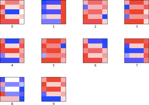
Fig 3. Matrix W at 100% accuracy.

The red color indicates positive interaction between the matrix and the image, while blue colors indicate negative interaction. Looking at 0, we can see that the model learned to distinguish between 0 and 8 by using negative weights for the line in the middle. For 1, the matrix strongly selects for a vertical line on the left, penalizing at the same time parts that would make the image look like 4, 7 or 9. 3 has positive interaction with almost all but 2 pixels, which would turn 3 into 8. The model did not learn the cleanest features, but it learned enough to tell each digit apart.

Clearly, linear regression can learn a number of features, given a well behaved problem. In the following posts we are going to show how a small change in the problem’s complexity causes linear regression to struggle. The change is to increase the image size, while keeping the digits sizes at 5. Deep neural networks are able to cope with this situation, at the expense of much longer training and much larger models. The final solution, that uses a convolutional neural network, can achieve fast training, 100% accuracy and small model size.

Resources

A Jupyter Notebook with the above code can be found at GitHub’s LCD repository.