machine learning, neural network

Dealing with inexact data

In the previous post we were dealing with an idealized setup. Each 5 by 5 digit fills completely a 5 by 5 image. In real world this is a very unusual occurrence. When processing images there is no guarantee that subjects completely fill them. The subject may be rotated, parts of it might be cut off, shadows may obscure it. The same applies to processing sounds. Ambient noises may be present, the sound we are interested in may not start right at the beginning of the recording, and so on. In this post we are going to show how adding a small degree of uncertainty can defeat an approach based on linear regression. We show how deep neural network can deal with this more complex task, at the expense of a much larger model and longer training time.

Adding uncertainty

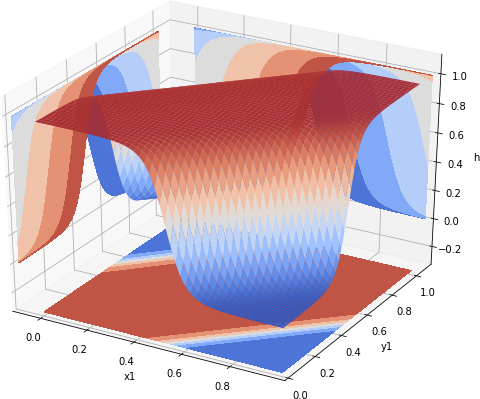
In order to simulate a real world setup we are going to slightly alter image generation. Previous image size and shape size were both set to 5. This way each shaped filled perfectly the entire image. There was no uncertainty as to where the image is located. Here we increase the image size to be twice the size of the shape. This leads to shape “jitter”, where the shape can be located anywhere in 10 by 10 grid, as shown in Fig 1.

10by10

Fig 1. LCD digits randomly located on a 10 x 10 grid.

Simple approach

We start by simply modifying img_size variable and running the same linear regression. Somewhat surprisingly, after 5 steps we hit 73% accuracy. When we complete the remaining steps, we reach 100% accuracy. It seems that this approach worked. However, this is not the case. Our linear regression learned perfectly the 100 examples we had. The mistake of the simple approach is not using any test data. Typically, when training a model, it is recommended that about 80% of data is used as training data, and 20% are used as test data. Fortunately, we  can easily rectify this. We generate another 50 examples, and evaluate accuracy for those. The result is 8%, or slightly worse than by a random chance. To see why this is the case, let us look at matrix W. Again, we reshape it as a 10 by 10 square, and normalize it within -1 to 1 value. The result is shown in Fig 2.

10by10-explain

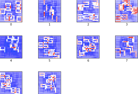
Fig 2. Matrix W at the end of training with 100 10×10 images

Now it is obvious that rather than learning how to recognize a given number, linear regression learned the location of each digit. If there is, say, 4 leaning against the left side of the image, it is recognized. However, once it is moved to the location not previously seen, the model lacks the means to recognize it. This is even more obvious if we run the training step with more examples. Rather than maintaining the accuracy, the quality of the solution quickly deteriorates. For example, if we supply 500 rather than 100 examples, the accuracy drops to 54%. Increasing the number of examples to 5,000 drops the accuracy to a dismal 32%. The confusion matrix shows that the only digit that the model learned to recognize is 1.

10by10-confusion

Fig 3. Confusion matrix for 5,000 examples.

Conclusions

Linear model is sufficient only for the most basic case. Even for a highly regular items, such as LCD digits, the model is not capable of learning to recognize them as soon as we permit a small “jitter” in the location of each digit. The above example also shows how important it is to have training and test data sets. Linear regression gave an impression of correctly learning each digits. Only by testing the model against independent test data we discovered that it learned positions of all 100 digits, not how to recognize them. This is reminiscent of case of a neural network that was trained to recognize between tanks camouflaged among trees and just trees (see Section 7.2. An Example of Technical Failure). It seemed to performed perfectly, until it was realized that photos of camouflaged tanks were taken on cloudy days, while all empty forest photos were taken on sunny days. The network learned how to recognize sunny from cloudy days, and knew nothing about tanks.

In the next installment we are going to increase the accuracy by creating a deep neural network.

Resources

You can download the Jupyter notebook from which code snippets and images were presented above from github linreg-large repository.

machine learning, neural network

Training neural net to emulate XNOR

In the last two posts we have shown how to encode, using Tensorflow, a neural network that behaves like the XNOR gate. However, it is a very unusual that we know, ahead of time, weights and biases. A much more common scenario is when we have number of inputs and the corresponding values, and wish to train a neural net to produce for each input the appropriate value. For us the inputs are (0, 0), (0, 1), (1, 0) and (1, 1). The values are 1, 0, 0, and 1. We have seen that a 2 layer deep neural network can emulate XNOR with high fidelity. Thus we could just create a 2 layer deep, 3 neuron network and attempt to train it. To facilitate some level of experimentation we create a function that produces a fully connected neural network layer.

def CreateLayer(X, width):
    W = tf.get_variable("W", [X.get_shape()[1].value, width], tf.float32)
    b = tf.get_variable("b", [width], tf.float32)
    return tf.nn.sigmoid(tf.add(tf.matmul(X, W), b))

The function creates X \times W + b input to a layer of neurons. Using X \times W instead W \times X allows us to specify n inputs (features) as a m \times n matrix. This is often easier than representing inputs as m columns each n high. Also, rather than creating variables directly, with tf.Variable, we use tf.get_variable. This allows variable sharing, as explained in Sharing Variables. It also can enhance display of the computation graph in TensorBoard, as explained in Hands on TensorBoard presentation.

We also create a training operation and a loss function that allows us to assess how well the current network is doing. Tensorflow offers a whole array of optimizers, but tf.train.AdamOptimizer is often a good choice. In order for the optimizer to push variables to a local minima we must create an optimizer operation. This is done by calling minimize method with a loss function. The loss function tells the optimizer how far it is from the ideal solution. We use the mean of squared errors as our loss function.

def CreateTrainigOp(model, learning_rate, labels):
    loss_op = tf.reduce_mean(tf.square(tf.subtract(model, labels)))
    train_op = tf.train.AdamOptimizer(learning_rate).minimize(loss_op)
    return train_op, loss_op

The above function returns the training and loss operations. The latter is used to track progress of the model towards the optimum. The final piece of code that needs to be written is the training code.

g = tf.Graph()
with g.as_default():
  X = tf.placeholder(tf.float32, [None, 2], name="X")
  y = tf.placeholder(tf.float32, [None, 1], name="y")
  with tf.variable_scope("layer1"):
    z0 = CreateLayer(X, 2)
  with tf.variable_scope("layer2"):
    z1 = CreateLayer(z0, 1)
  with tf.variable_scope("xnor"):
    training_op, loss_op = CreateTrainigOp(z1, 0.03, y)
  init_op = tf.global_variables_initializer()
  saver = tf.train.Saver()

X and y (line 3-4) are placeholders, which are going to be seeded with inputs and desired outputs. We specify the first dimension to be None to allow for arbitrary number of rows. In lines 5 – 10 we create a model. It consists of two, fully connected layers. The first layer has 2 neurons, the second consists of a single neuron. X is the input to the first layer, while the output of the first layer, z0, is the input to the second layer. The output of the second layer, z1 is what we wish to train to behave like the XNOR gate. To do so, in lines 9 and 10 we create a training operation and a loss op. Finally we create an operation to initialize all global variables and a session saver.

writer = tf.summary.FileWriter("/tmp/xnor_log", g)
loss_summ = tf.summary.scalar("loss", loss_op)

Before we run the training step we create a summary writer. We are going to use it to track the loss function. It can also be used to track weights, biases, images, and audio inputs. It also is an invaluable tool for visualizing data flow graph. The graph for our specific example is shown in Fig 1.

comp_graphFig 1. Data flow graph as rendered by tensorboard

In order to train our model we create two arrays representing features and labels (input values and the desired output). The training itself is done for 5,000 steps by the for loop. We feed the session all inputs and desired values, and run a training operation. What this does it runs the feed forward steps to compute z1 for the given inputs, weights and biases. These are then compared, using the loss function to the ideal responses, represented by y from these Tensorflow computes contributions all weights and biases make to the loss function. It uses the learning rate 0.03 to adjust them to make the loss smaller.

X_train = np.array([[0, 0], [0, 1], [1, 0], [1, 1],])
y_train = np.array([[1], [0], [0], [1]])

sess = tf.Session(graph=g)
sess.run(init_op)
for step in xrange(5000):
    feed_dict = {X: X_train, y: y_train}
    sess.run(training_op, feed_dict=feed_dict)
    if step % 10 == 0:
        writer.add_summary(
            sess.run(loss_summ, feed_dict=feed_dict), step)
save_path = saver.save(sess, '/tmp/xnor.ckpt')
sess.close()
print "Model trained. Session saved in", save_path

Once the training is complete we save the state of the session, close it and print the location of the single session checkpoint. The loss function, as recorded by the summary file writer, and rendered by TensorBoard, is shown in Fig 2.

loss
Fig 2. Loss function plotted by tensorboard.

At the end of the training it the loss function has the value of 0.000051287. It was still dropping but very slowly. In the next post we show how to restore the session and plot the loss function as well as the output of the trained neural network.

Resources

The Jupyter notebook that implements the above discussed functionality is xnor-train.ipynb in the xnor-train project.

machine learning, neural network

Using XNOR trained model

In the previous post we have described how to train a simple neural net to emulate the XNOR gate. The results of the training are saved as a solitary session checkpoint. In this post we show how to re-create the model, load the weights and biases saved to the checkpoint and finally plot the surface generated by the neural net over [0,1] x [0,1] surface.

tf.reset_default_graph()
X = tf.placeholder(tf.float32, [None, 2], name="X")
with tf.variable_scope("layer1"):
  z0 = CreateLayer(X, 2)
with tf.variable_scope("layer2"):
  z1 = CreateLayer(z0, 1)

We start by re-creating the model. For convenience, we added tf.reset_default_graph() call. Otherwise an attempt to re-execute this particular Jupyter cell results in error. Just like during the training method we create a placeholder for input values. We do not need, however, a placeholder for the desired values, y. Next, we re-create the neural network, creating two, fully connected layers.

saver = tf.train.Saver()
sess = tf.Session()
saver.restore(sess, "/tmp/xnor.ckpt")

The next three lines create a saver, a session, and restore the state of the session from the saved checkpoint. In particular, this restores the trained values for weights and biases.

span = np.linspace(0, 1, 100)
x1, x2 = np.meshgrid(span, span)
X_in = np.column_stack([x1.flatten(), x2.flatten()])
xnor_vals = np.reshape(
    sess.run(z1, feed_dict={X: X_in}), x1.shape)
sess.close()
PlotValues(span, xnor_vals)

The final piece of the code creates a 100 x 100 mesh of points from the [0,1] x [0,1] range. These are then reshaped to the shape required by X placeholder. Next, the session runs z1 operation, which returns values computed by the neural net for the given input X. As these are returned as 10,000 x 1 vector, we reshape them back to the grid shape before assigning them to xnor_vals. Once the session is closed, the values are plotted, resulting in surface shown in Fig 1.

xnor-trained-hd
Fig 1. Values produced by the trained neural net

The surface significantly different from the plots produced by Andrew Ng’s neural network. However, both of them agree at the extremes. To plot the values at the corner of the plane we run the following code:

print " x1| x2| XNOR"
print "---+---+------"
print " 0 | 0 | %.3f" % xnor_vals[0][0]
print " 0 | 1 | %.3f" % xnor_vals[0][-1]
print " 1 | 0 | %.3f" % xnor_vals[-1][0]
print " 1 | 1 | %.3f" % xnor_vals[-1][-1]

The result is shown below

  x1 | x2| XNOR
 ---+---+------
  0 | 0 | 0.996
  0 | 1 | 0.005
  1 | 0 | 0.004
  1 | 1 | 0.997

As it can be seen, for the given inputs the training produced the desired output. The network produces values close to 1 for (0, 0) and (1, 1) and values close to 0 for (0, 1) and (1, 0). If the above code is run multiple times, since weights and biases are initialized randomly, sometimes the trained network produces results that resemble those produced by Andrew Ng’s network.