In the previous post we have described how to train a simple neural net to emulate the XNOR gate. The results of the training are saved as a solitary session checkpoint. In this post we show how to re-create the model, load the weights and biases saved to the checkpoint and finally plot the surface generated by the neural net over [0,1] x [0,1] surface.

tf.reset_default_graph()
X = tf.placeholder(tf.float32, [None, 2], name="X")
with tf.variable_scope("layer1"):
  z0 = CreateLayer(X, 2)
with tf.variable_scope("layer2"):
  z1 = CreateLayer(z0, 1)

We start by re-creating the model. For convenience, we added tf.reset_default_graph() call. Otherwise an attempt to re-execute this particular Jupyter cell results in error. Just like during the training method we create a placeholder for input values. We do not need, however, a placeholder for the desired values, y. Next, we re-create the neural network, creating two, fully connected layers.

saver = tf.train.Saver()
sess = tf.Session()
saver.restore(sess, "/tmp/xnor.ckpt")

The next three lines create a saver, a session, and restore the state of the session from the saved checkpoint. In particular, this restores the trained values for weights and biases.

span = np.linspace(0, 1, 100)
x1, x2 = np.meshgrid(span, span)
X_in = np.column_stack([x1.flatten(), x2.flatten()])
xnor_vals = np.reshape(
    sess.run(z1, feed_dict={X: X_in}), x1.shape)
sess.close()
PlotValues(span, xnor_vals)

The final piece of the code creates a 100 x 100 mesh of points from the [0,1] x [0,1] range. These are then reshaped to the shape required by X placeholder. Next, the session runs z1 operation, which returns values computed by the neural net for the given input X. As these are returned as 10,000 x 1 vector, we reshape them back to the grid shape before assigning them to xnor_vals. Once the session is closed, the values are plotted, resulting in surface shown in Fig 1.

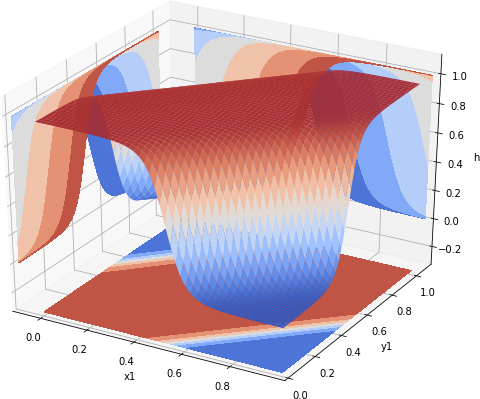
Fig 1. Values produced by the trained neural net

The surface significantly different from the plots produced by Andrew Ng’s neural network. However, both of them agree at the extremes. To plot the values at the corner of the plane we run the following code:

print " x1| x2| XNOR"
print "---+---+------"
print " 0 | 0 | %.3f" % xnor_vals[0][0]
print " 0 | 1 | %.3f" % xnor_vals[0][-1]
print " 1 | 0 | %.3f" % xnor_vals[-1][0]
print " 1 | 1 | %.3f" % xnor_vals[-1][-1]

The result is shown below

  x1 | x2| XNOR
 ---+---+------
  0 | 0 | 0.996
  0 | 1 | 0.005
  1 | 0 | 0.004
  1 | 1 | 0.997

As it can be seen, for the given inputs the training produced the desired output. The network produces values close to 1 for (0, 0) and (1, 1) and values close to 0 for (0, 1) and (1, 0). If the above code is run multiple times, since weights and biases are initialized randomly, sometimes the trained network produces results that resemble those produced by Andrew Ng’s network.