In Lecture 4.1 Linear Regression with multiple variables Andrew Ng shows how to generalize linear regression with a single variable to the case of multiple variables. Andrew Ng introduces a bit of notation to derive a more succinct formulation of the problem. Namely, 


For 

![\left[ \begin{array}{cccc} \theta_0 & \theta_1 & \cdots & \theta_n \end{array} \right] \times \left[ \begin{array}{ccccc} 1 & 1 & \cdots & 1 \\ x^{(1)}_1 & x^{(2)}_1 & \cdots & x^{(m)}_1 \\ & & \vdots \\ x^{(n)}_m & x^{(n)}_m & \cdots & x^{(n)}_m \\ \end{array} \right]](https://s0.wp.com/latex.php?latex=%5Cleft%5B+%5Cbegin%7Barray%7D%7Bcccc%7D+%5Ctheta_0+%26+%5Ctheta_1+%26+%5Ccdots+%26+%5Ctheta_n+%5Cend%7Barray%7D+%5Cright%5D+%5Ctimes+%5Cleft%5B+%5Cbegin%7Barray%7D%7Bccccc%7D+1+%26+1+%26+%5Ccdots+%26+1+%5C%5C+x%5E%7B%281%29%7D_1+%26+x%5E%7B%282%29%7D_1+%26+%5Ccdots+%26+x%5E%7B%28m%29%7D_1+%5C%5C+%26+%26+%5Cvdots+%5C%5C+x%5E%7B%28n%29%7D_m+%26+x%5E%7B%28n%29%7D_m+%26+%5Ccdots+%26+x%5E%7B%28n%29%7D_m+%5C%5C+%5Cend%7Barray%7D+%5Cright%5D+&bg=fffdfd&fg=606666&s=0&c=20201002)
is as close as possible to some observed values 


![i \in [1, m]](https://s0.wp.com/latex.php?latex=i+%5Cin+%5B1%2C+m%5D&bg=fffdfd&fg=606666&s=0&c=20201002)

To express the above concepts in Tensorflow, and more importantly, have Tensorflow find w. We are not using 
b to represent 
![h_{w,b}(X) = \left[ \begin{array}{ccc} \text{---} & (x^{(1)})^T & \text{---} \\ \text{---} & (x^{(2)})^T & \text{---} \\ & \vdots & \\ \text{---} & (x^{(m)})^T & \text{---} \end{array} \right] \times \left[ \begin{array}{c} w_1 \\ w_2 \\ \vdots \\ w_m \end{array} \right] + b](https://s0.wp.com/latex.php?latex=h_%7Bw%2Cb%7D%28X%29+%3D+%5Cleft%5B+%5Cbegin%7Barray%7D%7Bccc%7D+%5Ctext%7B---%7D+%26+%28x%5E%7B%281%29%7D%29%5ET+%26+%5Ctext%7B---%7D+%5C%5C+%5Ctext%7B---%7D+%26+%28x%5E%7B%282%29%7D%29%5ET+%26+%5Ctext%7B---%7D+%5C%5C+%26+%5Cvdots+%26+%5C%5C+%5Ctext%7B---%7D+%26+%28x%5E%7B%28m%29%7D%29%5ET+%26+%5Ctext%7B---%7D+%5Cend%7Barray%7D+%5Cright%5D+%5Ctimes+%5Cleft%5B+%5Cbegin%7Barray%7D%7Bc%7D+w_1+%5C%5C+w_2+%5C%5C+%5Cvdots+%5C%5C+w_m+%5Cend%7Barray%7D+%5Cright%5D+%2B+b+&bg=fffdfd&fg=606666&s=0&c=20201002)
This leads to the following Python code:
X_in = tf.placeholder(tf.float32, [None, n_features], "X_in")
w = tf.Variable(tf.random_normal([n_features, 1]), name="w")
b = tf.Variable(tf.constant(0.1, shape=[]), name="b")
h = tf.add(tf.matmul(X_in, w), b)
We first introduce a tf.placeholder named X_in. This is how we supply data into our model. Line 2 creates a vector w corresponding to b corresponding to h as a matrix multiplication of X_in and w plus scalar b.
y_in = tf.placeholder(tf.float32, [None, 1], "y_in")
loss_op = tf.reduce_mean(tf.square(tf.subtract(y_in, h)),
                         name="loss")
train_op = tf.train.GradientDescentOptimizer(0.3).minimize(loss_op)
To define the loss function, we introduce another placeholder y_in. It holds the ideal (or target) values for the function h. Next we create a loss_op. This corresponds to the loss function. The difference is that, rather than being a function directly, it defines for Tensorflow operations that need to be run to compute a loss function. Finally, the training operation uses a gradient descent optimizer, that uses learning rate of 0.3, and tries to minimize the loss.
Now we have all pieces in place to create a loop that finds w and b that minimize the loss function.
with tf.Session() as sess:
    sess.run(tf.global_variables_initializer())
    for batch in range(1000):
        sess.run(train_op, feed_dict={
            X_in: X_true,
            y_in: y_true
        })
    w_computed = sess.run(w)
    b_computed = sess.run(b)
In line 1 we create a session that is going to run operations we created before. First we initialize all global variables. In lines 3-7 we repeatedly run the training operation. It computes the value of h based on X_in. Next, it computes the current loss, based on h, and y_in. It uses the data flow graph to compute derivatives of the loss function with respect to every variable in the computational graph. It automatically adjusts them, using the specified learning rate of 0.3. Once the desired number of steps has been completed, we record the final values of vector w and scalar b computed by Tensorflow.
To see how well Tensorflow did, we print the final version of computed variables. We compare them with ideal values (which for the purpose of this exercise were initialized to random values):
print "w computed [%s]" % ', '.join(['%.5f' % x for x in w_computed.flatten()])
print "w actual   [%s]" % ', '.join(['%.5f' % x for x in w_true.flatten()])
print "b computed %.3f" % b_computed
print "b actual  %.3f" % b_true[0]

w computed [5.48375, 90.52216, 48.28834, 38.46674]
w actual   [5.48446, 90.52165, 48.28952, 38.46534]
b computed -9.326
b actual  -9.331
Resources
You can download the Jupyter notebook with the above code from a github linear regression repository.
 function. This function, abbreviated as XNOR, returns 1 only if
  . The values are summarized in the table below:
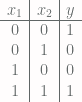
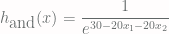


 . This way
 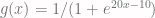 returns
  for
for  and
and  for
for  . By using −20 with both
  .
.