In Week 8 of Machine Learning Course, Andrew Ng introduces machine learning techniques for unlabeled data. These techniques allow one to discover patterns that exists in data, rather than train an algorithm to recognize an already known pattern. One algorithm frequently used to unearth natural grouping of data is k-means algorithm. When illustrating the workings of k-means algorithm for non-separated clusters Andrew Ng uses t-shirt sizing. Companies have to select, say four, t-shirt sizes, S, M, L, and XL. Each of the sizes has to accommodate some cluster of people. However, people do not come in discrete weight and height clumps. Instead, they form a continuum. We can see that by fetching some real-world data and using a scatter plot to show their distribution. Statistics Online Computational Resource (SOCR) provides a number of useful data sources. SOCR Data Dinov 020108 HeightsWeights set provides 25,000 records of human height and weight. For purposes of this tutorial we are going to rely on a smaller subset of 200 samples from that set. The distribution of data, plotted with matplotlib, is shown in Fig 1:
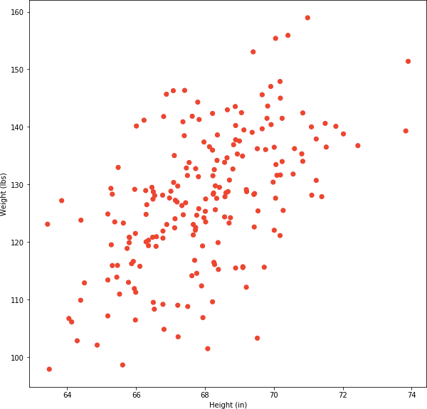
Fig 1. Scatterplot of 200 samples of human weight and height.
There is no obvious clusters visible in Fig 1. If we had to manually draw them, chances are that our choice would be sub-optimal. This is where k-means cluster algorithm comes to the rescue. Its objective is to find clusters 


In version 1.0.x of Tensorflow a number of new contribution libraries were introduced. Among them is the KMeansClustering estimator. It can be used to solve the t-shirt sizing problem in just a few lines of code. First, we need to define a function that provides data to the estimator. As there are various classes of estimators, ranging from linear regression, through neural networks to k-means estimator, the input function must return both features and labels. For k-means the labels are all None:
import pandas as pd

hw_frame = pd.read_csv(
  './hw-data.txt', delim_whitespace=True,
  header=None, names=['Index', 'Height', 'Weight'])
hw_frame.drop('Index', 1, inplace=True)

def input_fn():
  return tf.constant(hw_frame.as_matrix(),
                     tf.float32, hw_frame.shape), None
To simplify our task we use Pandas Data Analysis Library to load and transform data. We first read the SOCR file, and drop the index column. Then use the loaded data to return a 
Having constructed the input feed for the k-means estimator we create the estimator itself. We provide two parameters, the desired number of clusters and the loss tolerance. The second parameter allows us to let the estimator decide when to stop learning. When the loss function 
tf.logging.set_verbosity(tf.logging.ERROR)
kmeans = tf.contrib.learn.KMeansClustering(
    num_clusters=4, relative_tolerance=0.0001)
_ = kmeans.fit(input_fn=input_fn)
Once the estimator is created we ask it to fit the data, which, in case of k-means algorithm results in four clusters. We assign the return of fit function to a dummy variable _ to avoid Jupyter printing it as the output of the cell. Method fit returns the estimator itself, allowing for chaining of calls.
Once the clusters were computed all that is left is extracting their centers and indexes for all features points
clusters = kmeans.clusters()
assignments = list(kmeans.predict_cluster_idx(input_fn=input_fn))
Clusters are returned as 
numpy.ndarray, where k is the number of clusters and n is the number of features (2 in our case). Method predict_cluster_idx returns an iterable that for for each feature row returns the index of the cluster to which it is allocated. The outcome for SOCR data is shown in Fig 2.

Fig 2. Scatterplot clusters computed by k-means algorithm.
Resources
You can download a Jupyter notebook with the above code from and SOCR data from github kmeans repository.
